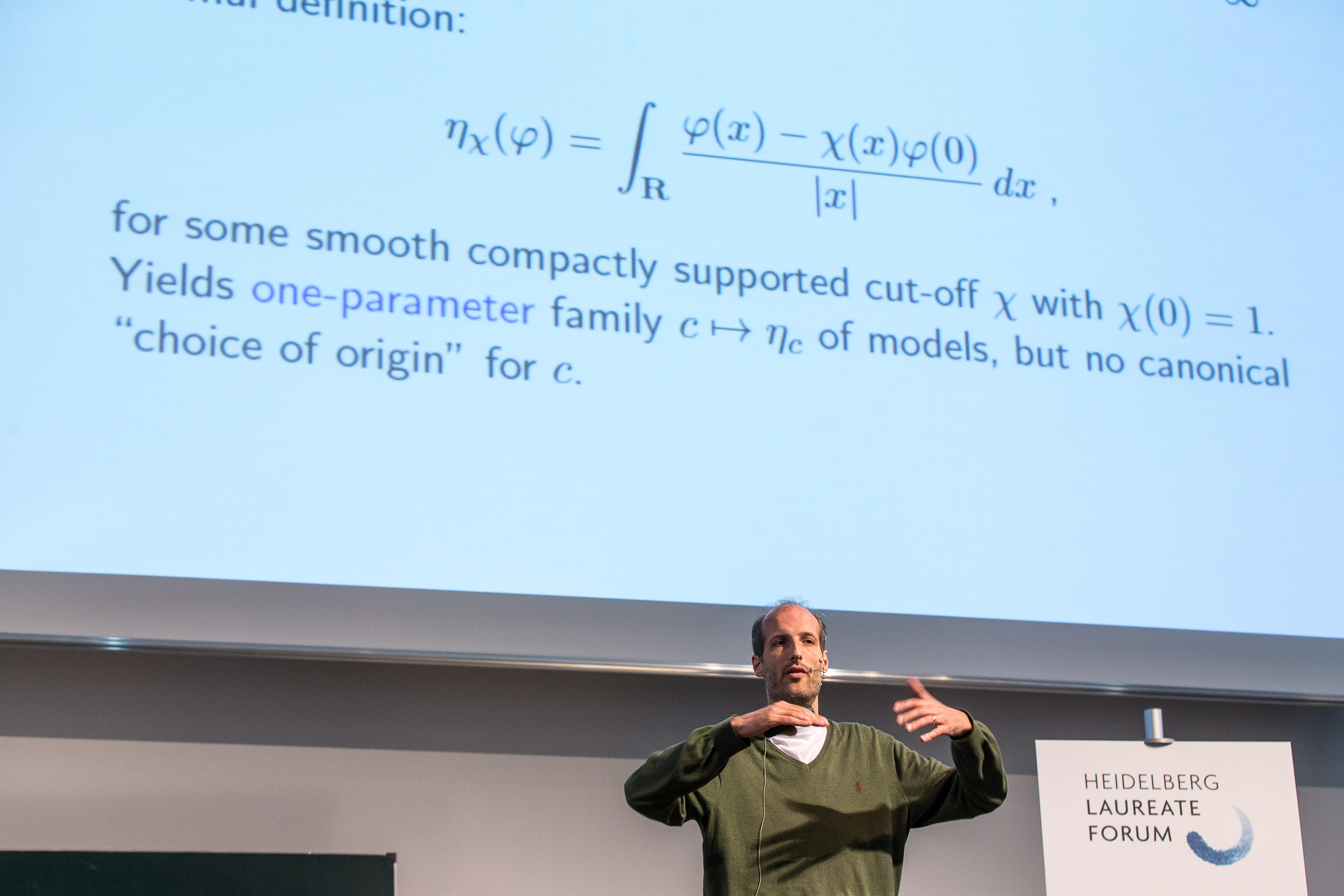
Martin Hairer’s talk on Tuesday, “Taming infinities”, was a fascinating tour of his main area of research, which combines random processes with mathematic’s preferred way of describing changing systems: differential equations. Trying to understand the basics of what Hairer was talking about was the most fascinating journey I’ve taken at this year’s HLF (so far!), and I want to (try and) share this with readers of the HLF blog. I won’t presume more than basic calculus, and even that will be used sparingly.

One caveat: When I write about cosmology, relativity, or astrophysics in general, I write about subjects I have spend a lot of time with. This is not such a subject – it is more of an attempt to capture incomplete glimpses into a world that is, to me, new and fascinating. Readers who know more about the subject matter are welcome to correct my statements and simplifications.

That said, to infinity and beyond:

Smooth physics

In classical physics, the way the world changes is described by differential equations that are nice and clean: Here is a particle with position x(t); its acceleration is determined by a given set of forces depending on the particle’s position, and possibly (friction!) its speed.

Most physics text books simply assume that the functions involved are continuous: they make no sudden jumps or anything like that. Usually, physicists go even further and assume that the way those functions change is also continuous (the functions are differentiable), and so is the way their change changes (higher derivatives), and so on. Often, for simplicity, it is assumed that all the higher-order rates of change are continuous, too, with not a jump in sight (“infinite differentiability”, also known as “smoothness”). This makes matters mathematically simple, and in most situation does not take anything away from the physical content of whatever model is under study.

What drives Brownian motion?

Most of the times, physicists get away with that. But sometimes they don’t. One famous case is Brownian motion as described statistically by Einstein. In its physical incarnation, Brownian motion was first observed by the botanist Robert Brown in the first half of the 19th century. Looking at pollen grains in water through his microscope, Brown noticed that the grains were moving ever so slightly, taking meandering paths that Brown could not explain at all.

The explanation was given by Einstein, in one of the papers published in his “miracle year” 1905: the pollen collide with the water molecules; the overall motion is the result of the sum of myriads of random collisions, and this hypothesis explains Brownian motion’s statistical properties (notably how far away from its starting point a pollen grain will have moved in a given amount of time, on average).

This nice animation, which can be found in the Wikipedia entry on Brownian motion, is a visualization of what’s going on, with the pollen grain in yellow and the molecules in black:

The equation describing the pollen grain’s motion is unusual, by physics standards. It is completely impractical to write down an equation that includes separate terms for each individual molecule that might be shoving around the pollen grain at some time or other.

What Einstein wrote down instead was an equation that did contain the usual derivatives of the pollen grain’s position (as one would expect in classical physics), but also a term that was unusual: It represented the random process of molecules colliding with the pollen grain. From a modern point of view, Einstein had written down the first stochastic differential equation, that is, the first differential equation incorporating random processes.

Brownian motion: The mathematician’s version

Stochastic differential equations are weird. The presence of randomness messes up many of the ordinary notions of differentiability, that is, of determining a quantity’s rate of change.

Brownian motion is an example – or more precisely: the version of Brownian motion used by mathematicians. In physics, if you look sufficiently closely, Brownian motion will resolve into ordinary motion of many, many molecules. When mathematicians talk about Brownian motion, they mean a version that is continuous in the same sense that fluids in fluid mechanics are continuous (whereas in real physics, a fluid is made of molecules or atoms): at whatever length scale you look, the probability of finding that, in a given time, your test particle (pollen grain) has moved a certain fraction of your length scale is given by a Gaussian probability distribution. This mathematically idealized Brownian motion is also known as the Wiener process, in honor of Norbert Wiener.

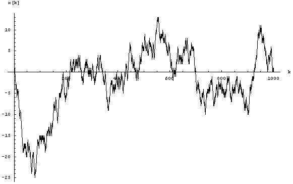
The following image shows an example where the particle can only move in one dimension:

In this image, the x axis represents the time, the y axis shows how far the particle has moved away from its starting point. The particle moves in the negative direction first, returning close to zero at time x=200, and so on.

A curve like this is easily extended to the right: just wait longer, and see where the particle goes in that time. Conceptually, in this way, you can extend the curve to infinity. There’s also a natural way of extending the curve to the left: Take a second Brownian motion curve that extends from x=0 to positive infinity, produce a mirror image by reflecting it at the y axis (now the curve extends from x=0 to negative infinity), and glue the two curves together. Voilà: Now you have two-sided Brownian motion.

The self-similarity of Brownian motion

Brownian motion has an intriguing property. If you zoom in, then what you will see will look basically the same as the original. Just by looking at the way the curve wiggles back and forth, you cannot tell at what “magnification” you are seeing the curve. This property is called self-similarity. Mathematically, the zooming-in involves scaling the x axis (time) by some c>0, and the why axis by one over square root of c. Here is a nice animation, similar to one that Hairer showed in his talk, which illustrates self-similarity:

As cool as this is, it is also problematic. This is not a smooth curve, it’s an exceedingly rough one. In a way, if we calculate a curve’s range of change, its derivative), what we are doing is “zooming” in until we are focused on a very small piece of the curve, which looks like part of a straight line. The slope of that straight line is the value of the curve’s derivative at that particular point.

Evidently, this won’t work for a Brownian curve. If we zoom in on such a curve, we’ll never see something resembling a straight line – only something resembling the original curve.

It is still possible to define something like a derivative in this curve. In a clearly defined sense, the derivative of Brownian motion is Gaussian white noise, that is, a curve that, at each point, has some random value determined by a Gaussian distribution (with the different values getting more and more improbable as they diverge further and further from zero).

As a result, this is not surprising – after all, this is the kind of change over time that was used to define the mathematical version of Brownian motion in the first place.

What is bound to be more surprising to most readers will be that, while the derivative of Brownian motion is defined, the square of the derivative is not. In fact, that square is infinite.

Excursion: Square road to infinity

How can that be? For numbers, or for ordinary functions, this would make no sense at all. If a number is finite, so is the square of that number; for the usual functions, where we can zoom in on one particular, well-defined function value at each point, the same statement holds true.

[If you know what Dirac’s delta function is, you’ll just need to recall that while the Delta function is well-defined, its square is not; feel free to jump over the rest of this section.]

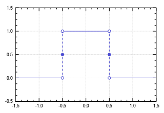
Imagine that I have a rectangular function, which has some constant value c in an interval between -b/2 and b/2 (for some constant b). The plot for this function will look like this (in this special case, b=c=1):

Choose bc=1, so the area under the curve – equivalently: the integral over the curve – is equal to one.

Now, make b>0 smaller and smaller, and keep bc=1, so the area under the curve – the integral over the curve – remains constant. For this process, there is a well-defined way of taking the limit of b going to zero. The function itself becomes highly problematic (and unplottable), since sending b to zero and keeping bc=1 means sending c to infinity in a carefully controlled way. The integral over the function remains well defined, since we took care to ensure that the area under the curve does not change: bc=1, throughout.

The function we obtain in the limit b to zero is the Dirac delta function, written as δ(x). Naively, it is non-zero only at x=0, and at x=0 it is infinite in just the right way to ensure that the integral over δ(x) gives the value 1.

What makes δ(x) highly useful is that, if we integrate not over δ(x), but over f(x)δ(x) with some ordinary function f(x), the result of the integral will be f(0), in words: the function value of f at x=0:

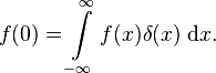
You can readily see this from our rectangular limit: If our rectangular function is very thin and tall, then f(x) will not vary all that much over the only part of the x-axis where the rectangular function isn’t zero. If our function is continuous (no jumps!), then its value all across the thin rectangle will not vary all that much, and in the integral, we can approximate f(x) by f(0). But this is just a constant factor in front of the integral – the remaining integral gives us the value 1, since that is the way our rectangle function was defined. The same reasoning carries over to the limit b to zero, that is: to the delta function.

A function like δ(x), which is not well-defined on its own (infinite at zero! zero everywhere else!), but which is well-defined as part of an integrand, is called a distribution.

What about the square of δ(x), then?

Naively, if the integral of any function multiplied by δ(x) gives that function, evaluated at x=0, then the integral of the square of δ(x) is

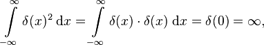
which is evidently ill-defined.

Here, then, is an example of a function – a distribution – that is well-defined (under the integral), but whose square is not well-defined and evaluates to infinity (again, under the integral).

Back to Brown

The situation for the square of the derivative of Brownian motion is the same. If you look more closely, stochastic differential equations are defined via integrals – just as in the case of the delta function.

And just as in the case of the delta function, if something is defined under an integral, its square can be ill-defined – for instance: infinite. This is what happens for the square of the derivative of Brownian motion.

In part 2, we’ll have a look at the applications for this type of rough curve that Hairer is interested in: Interfaces between different materials, or different phases of the same material.