In part 1 of “The rough worlds of Martin Hairer”, I explored some of the basics and some of the background behind stochastic differential equations, guided by the content of Martin Hairer’s HLF talk on Tuesday morning.

Now, it’s time to look at applications. And that is, at first sight, something completely different.

How to grow an interface

Imagine an interface, that is, a surface separating two different materials (or phases of the same material), as seen from the side in this sketch here:

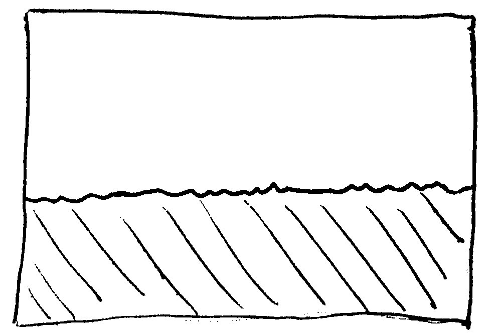
The two materials are stuff A (white) above, stuff B (hatched) below, the interface (wiggly line) in between separates the two.

There are situations in which region B will grow in a well-defined way. It could be that A is water and B is ice, and that the temperature is such that additional crystals will form, extending B. It could be that physicists are directing a molecular beam at a surface, depositing additional molecules at various places, extending B in this way. This is a situation that has quite a few incarnations.

If we just view a cross-section, as in the sketch above, or if we look at a simplified two-dimensional model in which what we see on the sketch is all that happens, the interface is a curve. So what curve, or what kind of curve is it?

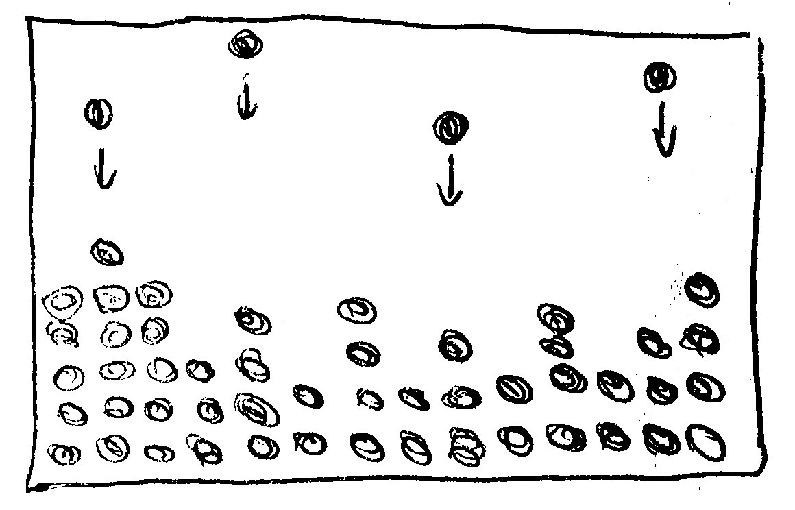
That, of course, depends on the details of the model. One type of growth model is known as ballistic: B-particles drop down in a random fashion; once they reach the existing surface (or, in some models, once they come close to a B particle that is already there), they stick.

I’ve tried to sketch this here; you see the existing B-stuff-area built up from columns of B particles (filled spheres), and some B particles raining down from above; in which column they fall is random:

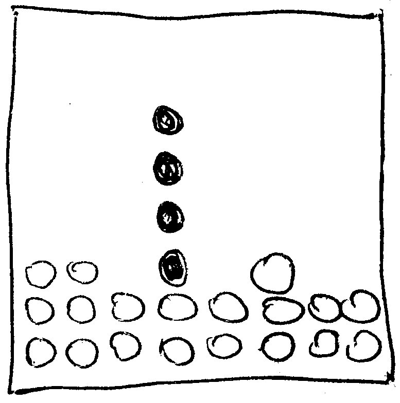
Some of the properties of this simple model are unphysical – they are unlikely to correspond to real system behaviour. For instance, now and again, this model will lead to rather thin and high columns sticking out from the surface, such as this (with the interesting B particles filled, the others not):

In reality, such fragile structures are unlikely to survive for long. Much more likely, the particles in question are going to spread out a bit – the high tower is going to sag:

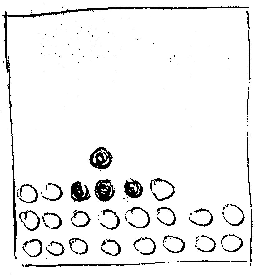
This is behaviour it makes sense to include in the interface growth model.

There is another somewhat unrealistic feature. In the model, the particles are falling from straight above. But if the interface (here once more drawn as a line) bulges upward already, as in the next sketch, we wouldn’t expect additional particle to adhere to it just from above:

Having the particles drop in from above is a simplification; in a realistic situation, we would expect there to be some particle accretion from a direction normal to the surface – in other words: in a direction at least partially lateral to the main “falling in” – as shown in this sketch here:

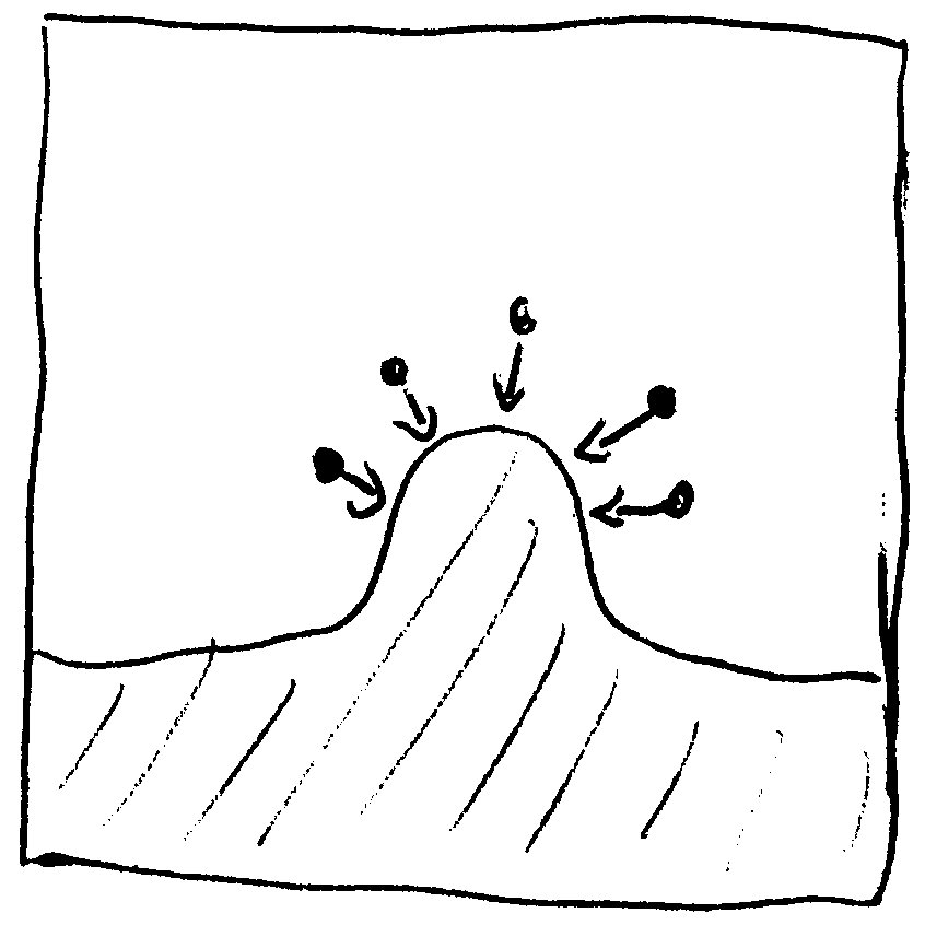
In other words: We would expect the interface not to grow strictly upward, as here…

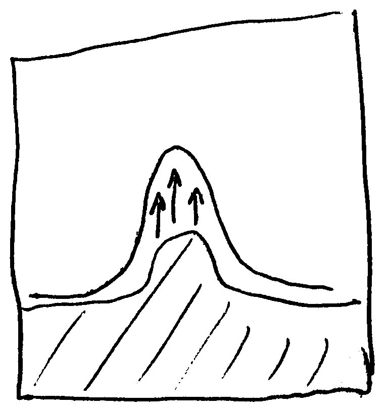
…but more as shown in the next sketch, outward from its present shape:

 

The KPZ model

A model of stochastic growth which incorporates all these features is the KPZ model, named after Mehran Kardar, Giorgio Parisi, and Yi-Cheng Zhang.

If the horizontal direction in all those sketches is chosen as the x direction, the model describes the interface curve by its height above the x axes, h(x,t).

In its full glory, the equation reads

The left-hand-side just tells us that this is an equation for how h(t,x), the interface curve, changes with time.

The terms on the right-hand-side incorporate the elements of the model we have discussed: the eta function describes the stochastic growth, namely the particles falling down to join the interface.

The second-order derivative with respect to x is the diffusion term – it makes sure that thin, high structures smooth out (“relax”) over time.

The square of the first derivative is responsible for “lateral growth”: making sure that a bump grows not strictly upward, but more outward from its present shape.

Brownian motion, KPZ and an infinity problem

So far, so good – but is the model even well-defined?

As it turns out, this presents a problem.

One can show, starting from a linearized form of the equation, showing that an interface that is already a Brownian motion curve will remain such a curve (though shifted upwards), and then going over to more general cases, that even if we start with an interface that is perfectly smooth to begin with, each part of it will evolve into something resembling a Brownian motion curve. The solutions to this equation are rough curves. Very rough.

The problem? We have seen that the square of the derivative of Brownian motion is ill-defined; put simply: it’s infinite. But the square of the derivative is a necessary part of the KPZ equation. The equation itself, taken at face value, is ill-defined!

Similar problem, similar solution: Renormalization for elementary particles

This, then, brings us to the title of the talk. These are the infinities to be tamed. They are not the only infinities to be tamed, though, since physicists encountered similar infinity problem – and solved it! – when trying to describe elementary particles.

Imagine that I’m trying to calculate how two electrons, which I am shooting towards each other in a particle accelerator, will react. In quantum field theory, the particle theory used for this kind of calculations, there are infinitely many contributions to what happens. Luckily, not all of them are equally important. In fact, the greater the number of particle reactions in one particular contribution, the smaller the contribution to the end result (which describes the statistics of how I can expect the two electron’s speeds and their directions to change during the encounter).

The most important contribution is represented by this diagram, known as a Feynman diagram and, in this case, read from bottom (past) to top (future):

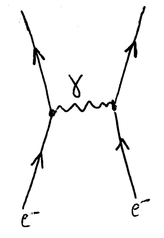
The two lines coming from below represent the two electrons. The wiggly line represents a photon (a “particle of light”) being exchanged between the two electrons. This contribution gives the same result as classical electrodynamics for the way the two electrons repel each other.

Here is an example for the next complicated version of what could happen – another Feynman diagram:

 

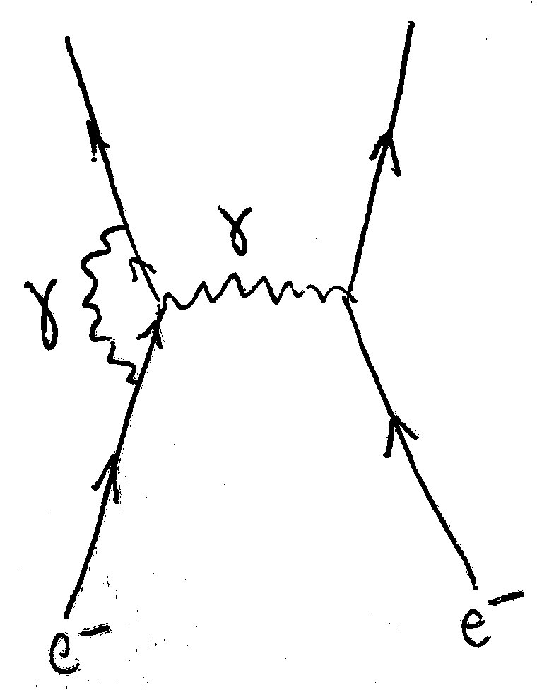
In this case, the electrons exchange two photons – there is another wiggly line on the left. This is a much rarer event than the first, and it will give a small correction to the way the electrons’ speeds and directions change.

Or, more precisely: taken at face value, it will not give a correction at all – it will kill the theory. If I calculate the contribution from this process, the result will be infinitely large, and that is certainly wrong. In particular, you get something like infinite masses or electric charges for your particles. The contribution is ill-defined – does this sound familiar?

Particle physicists have found a way around this problem. The basic gist is that the problem seems to arise because there is a sum (more precisely: an integral) that includes all the possible locations for the various interactions – including those where the interacting particles are infinitely close together. Should we really expect our theory to hold at all length scales? In physics, small length scales correspond to high energy scales. We certainly wouldn’t expect the theory to hold at all energy scales – at very high energies, there is a reasonable expectation for new physics to come into play.

This, then, is the way around the problem: Assume that the theory holds only up to a certain energy scale E which you are introducing by hand. (There are different possibilities for doing this.) Then, the result for the contribution remains finite, but explicitly depends on E. Re-define the parameters of your theory – the equations are of a form that allows for this – introducing new parameters that play the role of the masses and charges of your particles.

Now, compute the results that you can observe in an experiment – the aforementioned ways that speed and direction of motion of your electrons are likely to change as a result of the interaction. If you do this right, then you can now let E go back to arbitrarily high energies, and still retain a reasonable, finite result. You do have parameters for masses and charges to deal with, which need to be determined experimentally. But once you have determined these parameters, you get very good predictions for all additional reactions that you might encounter in your particle accelerator. Those predictions correspond to the experimental results with some of the highest degrees of precision achieved in physics, ever.

The procedure appears to work – and if you look back to what you have done, it appears as if you have subtracted, in a controlled way, infinity from your initial, ill-defined result. This has rendered your result finite and well-defined – at the cost of a few free parameters.

Saving KPZ

In fact, this procedure (known as “introducing counter-terms”) works for the KPZ equation as well: “subtract infinity” in a controlled way, and you obtain a well-defined equation, which you can then proceed to study.

There is an alternative way of viewing this which I found highly interesting. Ordinarily, if a function is differentiable, that is equivalent of viewing this function, at each point, as a polynomial (think “Taylor expansion”): the coefficient of the linear term is the value of the derivative of the function at the point in question, the coefficient of the quadratic term is half of the value of the second derivative at this point, and so on.

Recall that the problem in the case of solutions of the KPZ equation – and in the case of Brownian motion – was the stochastic nature of the term describing the random particles contributing to the growth of the interface. This resulted in ill-defined derivatives (or squares therof). In the Brownian motion case, this was obvious: Zoom in, and self-similarity will make sure that what you see will never approach anything that looks linear, or like a simple polynomial.

Hairer talked about the possibilities of writing such functions in a different way – not in terms of polynomials, but in terms of functions that show similarly weird behaviour. (In fact, the Brownian motion functions are good candidates for parts of such a new basis!) In this new basis, any given function would be characterized by the coefficients in front of the basis function – just as in the ordinary case, where the basis functions are monomials.

The cool thing is that, in this unusual basis, you could do pretty much all of the things you would also do with the ordinary polynomial (Taylor) decompositions. In the new basis, too, the coefficients would play the role of values of the derivative. The basis functions could be ordered by their degree, just like monomials, so a series development would have similar properties (including that you could develop up to a certain point, and then neglect smaller terms).

All this seemed to me to be a weird way to recover from these stochastically handicapped functions the properties that ordinary physicists love and cherish in the more usual functions they are used to.

Conclusion

I have not yet covered all of Hairers talk – notably, there were interesting conjectures about whether or not “zooming out” on any interface that arises not only from the KPZ equation, but from other, related models will always end up, asymptotically, with a universal, self-similar solution of the Brownian motion type – but I will stop here. I believe that what I have written captures the basics of Hairers talk. All in all, for me, the talk was what HLF should be all about: Opening up new worlds – even if you are allowed only a tantalizing, incomplete glimpse.

Later addition: Hairer’s talk slides can be found on this web pages, here.